DV-Solve: A Random-First Solver
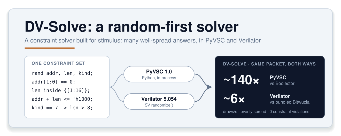
The last post ended with “Next time: the solver.” This is that post. It covers why constrained-random stimulus needs a solver of its own, what dv-solve is, and how to turn it on from PyVSC and from Verilator, with numbers from one small example run both ways. It ends with how we check that dv-solve’s answers are right, and how you can run the same check on your own tests.
Existing PyVSC code runs on dv-solve unchanged. Where Boolector is installed, Boolector stays the default, and switching to dv-solve takes one line.
Why constrained random needs a different solver
Constrained randomization is central to how we verify hardware. Instead of listing test cases, we describe what’s legal and let a solver choose. A constraint set is easier to review than a list of cases, and it keeps working as the design changes. Paired with coverage goals, it also answers a question a list of tests can’t: is everything I care about reachable?
It isn’t only a simulation technique, either. riscv-dv generates random instruction streams. Its main generator is written in SystemVerilog, largely so that it can use the simulator’s solver, and its Python generator is built on PyVSC. Microsoft’s DatagenDV builds test stimulus on PyVSC. PSS tools generate whole tests from constraints, and many flows generate configurations the same way.
The open-source solvers we have for this work were built for a different job. SAT and SMT solvers come out of formal verification and software analysis, where the question is whether a solution exists. They are very good at answering it. Stimulus generation asks for something else.
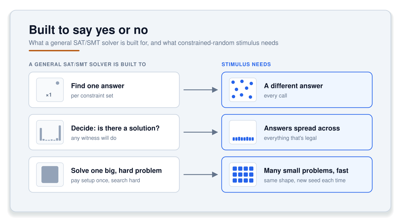
Two consequences of that mismatch shaped dv-solve. The first is that most of
the work is easy. Bounds, ranges and set membership make up the bulk of real
stimulus constraints, and running a general decision procedure on every call
taxes all of them. The second is that the first answer a solver finds is a
poor sample. Solvers tend to land near the edges of the space. The
inside {1, 2, [100:200]} histogram in the last
post shows the result: stock PyVSC
put half of 4,000 draws on two values.
Simulators face the same problem. Verilator’s randomize() hands
constraints to an external SMT solver, and Verilator then has to issue
extra queries of its own to get varied answers back. Verilator 5.054 adds
an option to leave the sampling to the solver instead, which we’ll use
below.
What dv-solve is
dv-solve is a constraint solver built for stimulus from the start. Its job
is to get the spread of answers right, not to accept whatever falls out of
the search. It’s Apache-2.0 licensed and installs with
pip install dv-solve. The current release is 0.5.0.
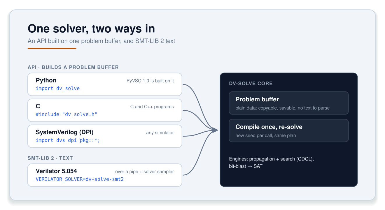
There are two ways in. The first is an API, with bindings for C
(dv_solve.h), Python (the dv_solve package, which PyVSC is built on)
and SystemVerilog (DPI packages that work on any simulator). Every binding
describes a problem the same way, as a single contiguous problem buffer.
A buffer is plain data. It can be copied or saved, and there’s no text to
parse on each call. You compile it once, then re-solve it with a new seed
every time you need a value. The DPI route shows what that allows: the
problem is built in Python ahead of time and embedded in a SystemVerilog
package, so the testbench only compiles and solves.
The second way in is SMT-LIB 2 text, read by the dv-solve-smt2 command
(the QF_BV, QF_ABV, QF_UFBV and QF_AUFBV logics). That’s how Verilator
talks to dv-solve today. Having Verilator emit problem buffers when it
compiles the design is the next step, and that work is at the design stage.
The core is plain C. The C++ parts (the CaDiCaL SAT solver) are optional, so building it needs only a C compiler.
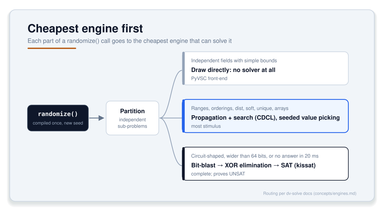
Inside, dv-solve tries the cheapest engine first. Each problem is split into independent sub-problems, and each sub-problem goes to the cheapest engine that can solve it:
- No solver at all. Independent fields with simple bounds are drawn
directly, in PyVSC’s front-end. This tier exists because we measured it:
building and solving a problem of unconstrained fields in the native
solver on every call was 4x slower than calling Python’s
randint. - Propagation and search. Most stimulus constraints go here: ranges,
orderings,
dist,soft,uniqueand arrays. The engine narrows each field’s domain by propagation, searches (CDCL), and uses the seed to choose values. - Bit-blasting to SAT. The rest is translated to a SAT problem and solved with kissat. That covers fields wider than 64 bits, circuit-shaped problems, searches the propagation engine can’t finish (for SMT-LIB input, within 20 ms), and proving that a problem has no solution.
If Boolector is installed, PyVSC can still fall back to it for a handful of shapes. Over the course of this work, fallback events across PyVSC’s test suite went from 1,419 to 5.
Partitioning and compiling once are most of why dv-solve is fast in a testbench, where the same object is randomized thousands of times.
One example, two front-ends
The example is a bus packet: a word-aligned address in the first 4 KB, a
length from 1 to 16, and a kind field where kind 7 requires a long packet.
Below it is written once for PyVSC and once in SystemVerilog. dv-solve gets
the same problem either way.
PyVSC (1.0 and later)
Installing PyVSC brings dv-solve with it. On Linux x86_64 and macOS it also brings Boolector, which stays the default there, so dv-solve is opt-in. On Windows and Linux aarch64, dv-solve is the default.
pip install pyvsc # 1.0.0 or later; installs dv-solve tooOne call selects dv-solve:
import vsc

vsc.set_solver_backend("dv-solve")     # or: export VSC_SOLVER=dv-solve

@vsc.randobj
class Packet(object):
    def __init__(self):
        self.addr = vsc.rand_bit_t(32)
        self.len  = vsc.rand_bit_t(8)
        self.kind = vsc.rand_bit_t(4)

    @vsc.constraint
    def c_align(self):
        self.addr[1:0] == 0

    @vsc.constraint
    def c_len(self):
        self.len.inside(vsc.rangelist(vsc.rng(1, 16)))

    @vsc.constraint
    def c_fit(self):
        self.addr < 0x1000
        self.addr + self.len <= 0x1000

    @vsc.constraint
    def c_kind(self):
        self.kind != 0
        with vsc.implies(self.kind == 7):
            self.len > 8

print("solver backend:", vsc.get_solver_backend())   # -> dv-solve
p = Packet()
for _ in range(5):
    p.randomize()
    print(f"addr={p.addr:08x} len={p.len} kind={p.kind}")
Nothing is logged when the backend changes, so vsc.get_solver_backend() is
the way to check which one is active. Setting VSC_SOLVER=dv-solve in the
environment does the same thing without editing the code.
If you adapt this example, watch the inside constraint.
vsc.rangelist([1, 16]) means the two values 1 and 16, not the range
between them. For a range, use vsc.rng(1, 16) or the tuple (1, 16). I
made exactly this mistake writing the example, and for a few minutes it
looked like a solver bug.
Verilator (5.054 and later)
Verilator’s randomize() runs an external SMT-LIB solver as a subprocess,
and dv-solve can be that solver. Here is the same packet in SystemVerilog:
class Packet;
  rand bit [31:0] addr;
  rand bit [7:0]  len;
  rand bit [3:0]  kind;

  constraint c_align { addr[1:0] == 2'b00; }             // word aligned
  constraint c_len   { len inside {[1:16]}; }
  constraint c_fit   { addr < 32'h1000; addr + 32'(len) <= 32'h1000; }  // in the first 4 KB
  constraint c_kind  { kind != 0; (kind == 4'd7) -> (len > 8); }
endclass

module top;
  initial begin
    automatic Packet p = new;
    repeat (5) begin
      if (p.randomize() == 0) $fatal(1, "randomize() failed");
      $display("addr=%h len=%0d kind=%0d", p.addr, p.len, p.kind);
    end
    $finish;
  end
endmodule
Two settings matter:
VERILATOR_SOLVER=dv-solve-smt2selects the solver. No other flags are needed.+verilator+rand+sampler+solveron the simulation command line (orVERILATOR_RAND_SAMPLER=solverin the environment) is the option 5.054 added (verilator#8899). It passes the solver a seed and lets the solver do the sampling, in place of the extra queries Verilator would otherwise make.
Prebuilt Verilator 5.054 binaries for Linux (x86_64 and aarch64), macOS (arm64) and Windows are on the edapack/verilator-bin release page. They use Bitwuzla as the default solver. dv-solve installs separately, with pip, and Verilator needs dv-solve 0.5.0 or later.
pip install 'dv-solve>=0.5.0'            # puts dv-solve-smt2 on PATH
verilator --binary packet.sv
export VERILATOR_SOLVER=dv-solve-smt2
./obj_dir/Vpacket +verilator+rand+sampler+solver +verilator+solver+file+solver.log
grep -E '^# Open|; sampler' solver.log   # "# Open: dv-solve-smt2" / "; sampler: solver"
The solver log records which solver ran and which sampler it used, and the
grep pulls out both lines. If Verilator can’t start the solver, it prints
%Warning: Unable to communicate with SAT solver and randomize() returns 0.
The solver sampler is an option rather than Verilator’s default because it only helps with a solver that uses the seed to vary its answers. dv-solve does, so use the two together.
What it buys you
The numbers below come from drawing the packet over and over from one
object. Each configuration ran with three seeds: 20,000 draws per seed in
PyVSC and 5,000 in Verilator. PyVSC timing counts only the randomize()
calls. Verilator timing is the wall time of the whole simulation, so it
includes start-up and the solver subprocess. Each dv-solve result is
compared with what you get out of the box.
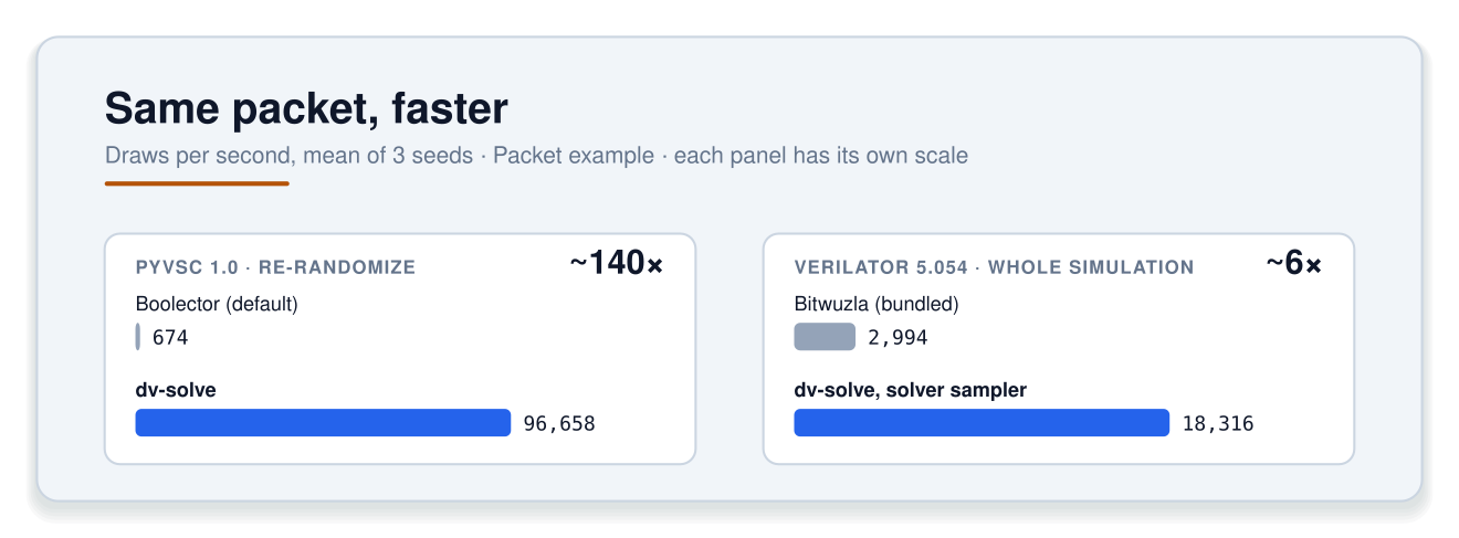
In PyVSC, dv-solve draws about 96,700 packets a second to Boolector’s 674, roughly 140x. That’s one small class re-randomized in place, which is the best case for compile-once, so don’t expect 140x across the board. On the broader PyVSC benchmark suite, unchanged classic code re-randomizes about 58x faster and creates new objects about 2.7x faster. Array-heavy code that builds a new object for every randomization gains little, about 1.1x.
Under Verilator, dv-solve with the solver sampler runs at about 18,300 draws a second, against 3,000 for the default Bitwuzla setup. That’s about 6x, measured on the whole simulation.
Speed is only half the result. To measure spread, we enumerated every legal
packet, worked out what share of draws each value of len, kind and the
address page would get under a uniform pick, and compared the draws against
that. A true uniform sample of the same size shows how much difference is
just sampling noise.
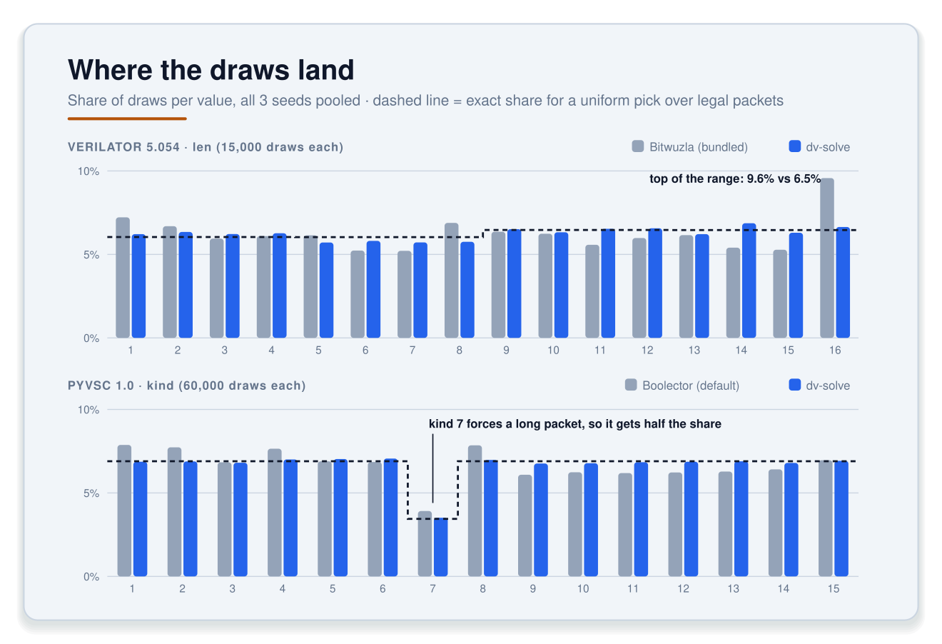
dv-solve stays within that noise on every field, in both front-ends. The
default Bitwuzla setup over-picks len = 16, and Boolector leans toward
kinds 1 through 8. Every run produced zero constraint violations, checked
independently in Python.
Better on relational constraints
The last post showed dv-solve doing badly on SyoSil’s uniformity test
(x <= y over [0:9], 10,000 draws), with only 12 of the 55 cells
within 10% of the ideal share and the two corner cells drawn nearly three
times too often. Relational constraints were the next thing to fix.
dv-solve now tries a uniform draw before it searches. It draws every related field at once from its range, checks the constraints, and keeps the draw if it fits. A draw accepted that way is exactly uniform over the solutions. After a few misses, or when legal values are too sparse for draws to hit them often, it searches as before. Here is the same test on the current releases, PyVSC 1.0.0 and dv-solve 0.5.0:
| Cells within 10% | Busiest cell (ideal 1.82%) | |
|---|---|---|
| Stock PyVSC 0.9.6 + Boolector | 15 of 55 | 3.4% |
| PyVSC + dv-solve (last post) | 12 of 55 | 5.2% |
| PyVSC 1.0.0 + dv-solve 0.5.0 | 52 of 55 | 2.0% |
| constrainedrandom | 46 of 55 | 2.2% |
Don’t read too much into 52 against 46. At 10,000 draws, a perfectly uniform sampler would land about 45 cells within 10%, so both are within sampling noise of uniform. The point is that dv-solve no longer stands out. The grid also runs in PyVSC’s CI now, as a gate, so this result can’t quietly regress.
a < b over 8-bit values shows the same change. The ideal mean of a is
84.7; dv-solve now gives 84.4, and Boolector 101.8.
How do we know it’s right?
A new solver is a new place for wrong answers to hide. A generator that quietly violates a constraint is worse than a slow one, because nothing tells you it happened. dv-solve’s answers are checked in three ways:
- XCHECK runs Boolector alongside dv-solve. Each dv-solve answer must satisfy the constraints, and the two solvers must agree on whether a solution exists.
- VALIDATE re-checks every answer against the constraints, in CI.
- An independent oracle checks answers with z3. Across the classic and dataclass test suites, it agreed with all 34,980 of them. It checks the engine, not PyVSC’s translation into it.
Two bugs found along the way show why there are three.
In the first, with dv-solve as the default backend, if/else constraints
were violated 63% of the time, with no error. The guard logic was fine. The
cause was a width-extension wrapper around one leaf of an OR expression.
At the time, only XCHECK caught it. VALIDATE was added afterwards, and it
catches this bug too.
In the second, c32 == a16 + b16 dropped the carry about 47% of the time,
but only on machines without Boolector. When Boolector was installed, PyVSC
routed that shape to it, and CI always had Boolector installed, so CI never
saw the bug. Users without Boolector would have. The lesson was to test
the configuration users actually run, and a CI job with no Boolector now
gates every PyVSC release.
Checking your own workloads
The last post promised a way to run these checks on your own tests. It’s an environment variable:
VSC_SOLVER=dv-solve VSC_DVSOLVE_XCHECK=1 python my_test.pyWith XCHECK on, every dv-solve answer is checked against Boolector. It
doesn’t re-solve, so the values your test sees don’t change. The first
disagreement raises XCheckMismatch. VSC_DVSOLVE_XCHECK_WARN=1 logs and
counts mismatches instead of raising, and VSC_DVSOLVE_XCHECK_RATE=0.1
checks one answer in ten. The cost is modest. On the packet example,
dv-solve with XCHECK still ran at about 2,900 draws a second, roughly 4x
Boolector on its own.
XCHECK needs Boolector, which PyVSC installs on Linux x86_64 and macOS.
Without Boolector, the checks are skipped and nothing tells you, so check
that import pyboolector works before relying on a clean run.
What PyVSC stops depending on
Boolector is now optional: PyVSC imports and runs without it. It’s still useful as the cross-check oracle and as the fallback for a few shapes, so it isn’t going away.
The change matters most for installation, since the Boolector Python package has been the hardest part of installing PyVSC on some platforms. dv-solve ships wheels for Linux (x86_64 and aarch64), macOS (arm64 and x86_64) and Windows (AMD64), one wheel per platform that works with any Python 3 version. PyVSC 1.0 requires dv-solve on every platform and Boolector only on Linux x86_64 and macOS, which is why dv-solve is already the default on Windows and Linux aarch64.
Where it falls short
- constrainedrandom is still faster on simple problems. On
constrainedrandom’s own benchmark suite, PyVSC’s dataclass front-end on
dv-solve (the subject of the next post) is 2.0x faster re-randomizing one
object and 3.7x faster creating a fresh object each time. On our broader
suite the two are even with fresh objects, and constrainedrandom is about
1.7x faster re-randomizing. It wins on loosely constrained shapes and on
weighted
dist. - There are known gaps.
arr.productisn’t supported. A couple of small UNSAT cases with symbolic array indices, and fields wider than 255 bits, still need Boolector. When a solve fails,solve_fail_debuglists every hard constraint rather than the smallest conflicting set.
We’re not making any comparison with the solvers in commercial simulators.
A new solver is necessary, not sufficient
The riscv-dv numbers from the last post put the solver in proportion. Switching to dv-solve took pygen from 128 to 474 instructions a second, with no changes to pygen. Most of the remaining distance to 13,569 came from changing the model. Porting pygen’s instruction classes to the dataclass front-end was worth 13.8x by itself. A faster solver can’t remove work the front-end does before the solver is ever called.
That’s the subject of the next post: dataclasses, where structure is set up once per class instead of once per object.
Closing
A solver improves the way other open-source tools do: people run it on their own problems and report what they find. A few specific requests:
- Run your PyVSC tests with
VSC_DVSOLVE_XCHECK=1and send us anything it flags. - Send us constraint shapes, especially ones where the distribution looks wrong. Distribution bugs stay hidden until someone measures them, and constrainedrandom’s benchmark suite has already made this solver better.
- Try the Verilator path on your own SystemVerilog and tell us how it goes.
Issues go to fvutils/dv-solve or fvutils/pyvsc. Each shape someone reports becomes a test. And because every front-end shares one solver, a fix for a shape one Python user reports also reaches people randomizing in SystemVerilog.
Next time: dataclasses.